Comparison of Tidal Modes

In this demo we will show the relative strength of various tidal modes by looking at the eccentricity functions.

import numpy as np
import matplotlib.pyplot as plt

# Choose which l you want to look at. Here we will look at l=2
max_l = 5
from TidalPy.tides.eccentricity_funcs import orderl5 as eccen_funcs

eccentricity_domain = np.linspace(0., 0.9, 100)

# Choose which truncation level to use. Here we will look at truncation level 6
eccentricity_results = eccen_funcs.eccentricity_funcs_trunc20(eccentricity_domain)

# Plot the results by collapsing all "q" results into a single value.
fig_p_compare, ax_p = plt.subplots(figsize=(8,6))
fig_q_compare, ax_q = plt.subplots(figsize=(8,6))
ax_p.set(xlabel='Eccentricity', xscale='linear', ylabel='Terms of $G^{2}_{l=' + f'{max_l}' + ',p,q}$', yscale='log')
ax_q.set(xlabel='Eccentricity', xscale='linear', ylabel='Terms of $|G^{2}_{l=' + f'{max_l}' + ',p=' + f'{max_l}' + ',q}|$', yscale='log')
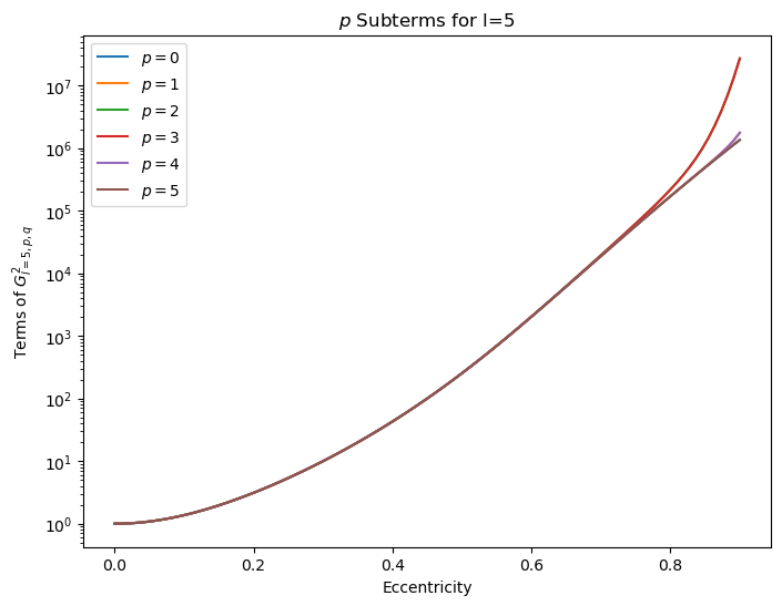
ax_p.set(title=f'$p$ Subterms for l={max_l}')
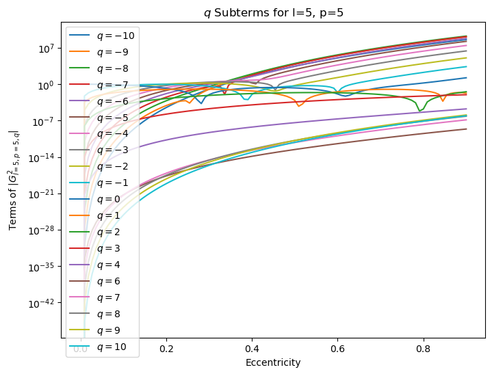
ax_q.set(title=f'$q$ Subterms for l={max_l}, p={max_l}')
for p in range(max_l+1):
    q_collapsed = 0.
    for q, q_res in eccentricity_results[p].items():
        if p == max_l:
            ax_q.plot(eccentricity_domain, np.abs(q_res), label='$q=' + f'{q}' + '$')
        q_collapsed += q_res
    ax_p.plot(eccentricity_domain, q_collapsed, label='$p=' + f'{p}' + '$')

ax_p.legend(loc='best')
ax_q.legend(loc='best')
plt.show()